Thermodynamic Properties of the Quantum Harmonic Oscillator
Introduction
The quantum harmonic oscillator is one of the staple problems in quantum mechanics. It has that perfect combination of being relatively easy to analyze while touching on a huge number of physics concepts. Additionally, it is useful in real-world engineering applications and is the inspiration for second quantization and quantum field theories.

Most introductory quantum mechanics courses stop the analysis of the quantum harmonic oscillator at finding the energy levels of the different energy eigenstates. However, we can do so much more! The simple structure of the energy levels allows us to easily compute some of the thermodynamic properties of the quantum harmonic oscillator. Let’s take a look.
The Partition Function
If we want to study the thermodynamic properties of the quantum harmonic oscillator, then it makes sense to start our analysis with the derivation of the partition function. This is a quantum mechanical system with discrete energy levels; thus, the partition function has the form:
\[\begin{equation} Z = Tr \left ( e^{-\beta \hat{H}}\right ) \end{equation}\]In the expression above, \(\hat{H}\) is the Hamiltonian of the system while \(\beta\) is the thermodynamic beta. Normally, taking the trace of a matrix exponential is a long and painful process. However, we can easily calculate this sum if we choose eigenvectors in the energy basis. The quantum harmonic oscillator has an infinite number of energy levels, indexed by the letter n.
\[\begin{align} Z &= Tr \left ( e^{-\beta \hat{H}} \right )\\[0.1cm] &= \sum_{n=0}^\infty \left \langle n \right | e^{-\beta \hat{H}} \left | n \right \rangle\\[0.1cm] &= \sum_{n=0}^\infty e^{-\beta E_n}\\[0.1cm] \end{align}\]Students of quantum mechanics will recognize the familiar formula for the energy eigenvalues of the quantum harmonic oscillator.
\[\begin{equation} E_n = \left ( n + \frac{1}{2} \right ) \hbar \omega \end{equation}\]Plugging this expression for energy into the partition function yields:
\[\begin{align} Z &= \sum_{n=0}^\infty e^{-\beta \left ( n + \frac{1}{2} \right ) \hbar \omega}\\[0.1cm] &= \sum_{n=0}^\infty e^{-\beta n \hbar \omega}e^{-\beta\hbar\omega/2}\\[0.1cm] &= e^{-\beta\hbar\omega/2} \sum_{n=0}^\infty e^{-\beta n \hbar \omega}\\[0.1cm] &= e^{-\beta\hbar\omega/2} \sum_{n=0}^\infty \left ( e^{-\beta \hbar \omega} \right )^n \end{align}\]The product \(\beta \hbar \omega\) is always positive, so the exponent in the sum is always going to be less than one. Thus, we can sum this exponent using a geometric series:
\[\begin{equation} \sum_{n=0}^\infty x^n = \frac{1}{1 - x} \end{equation}\]The partition function becomes:
\[\begin{align} Z &= e^{-\beta \hbar \omega/2} \left ( \frac{1}{1 - e^{-\beta \hbar \omega}} \right )\\[0.1cm] &= \left ( \frac{1}{e^{\beta \hbar \omega/2}} \right ) \left ( \frac{1}{1 - e^{-\beta \hbar \omega}} \right )\\[0.1cm] &= \frac{1}{e^{\beta \hbar \omega/2} - e^{-\beta \hbar \omega/2}}\\[0.1cm] \end{align}\]If you want to be really fancy, you can write the partition function in terms of a hyperbolic cosecant.
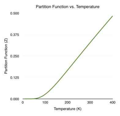
\[\begin{equation} Z = \frac{1}{e^{\beta\hbar\omega/2} - e^{-\beta\hbar\omega/2}} = \frac{1}{2} csch \left ( \frac{\beta \hbar \omega}{2} \right ) \end{equation}\]For me personally, a hyperbolic cosecant is all flash and no substance. We need to take derivatives and logorithms of the partition function in order to find the different thermodynamic properties. It is much easier to do that when the partition function is in terms of exponents instead of inverse hyperbolic functions! Shown below is a plot of the partition function versus temperature (T). I set \(\hbar \omega = 1 \times 10^{-20}\) J, corresponding to oscillations (\(\omega\)) in the infrared light frequency.
Helmholtz Free Energy
Once I get the partition function for a system, I like to calculate the Helmholtz free energy next. It usually is a pretty quick calculation, and it can be used as a stepping stone for future thermodynamic quantities. The definition of the Helmholtz free energy is:
\[\begin{equation} F = -\frac{1}{\beta} ln(Z) \end{equation}\]Since products can be separated within logarithms, I will use this slight raw form of the partition function rather than the final expression we got above:
\[\begin{equation} Z = e^{-\beta \hbar \omega/2} \left ( \frac{1}{1 - e^{-\beta \hbar \omega}} \right ) \end{equation}\]This will make the final expression look much nicer. Plugging in the expression for \(Z\) and simplifying yields:
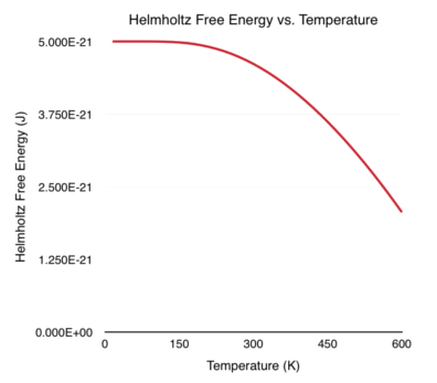
\[\begin{align} F &= -\frac{1}{\beta} ln \left [ e^{-\beta \hbar \omega/2} \left ( \frac{1}{1 - e^{-\beta \hbar \omega}} \right ) \right ]\\[0.1cm] &= -\frac{1}{\beta} ln \left ( e^{-\beta \hbar \omega/2} \right ) -\frac{1}{\beta} ln \left ( \frac{1}{1 - e^{-\beta \hbar \omega}} \right )\\[0.1cm] &= -\frac{1}{\beta} \left (-\frac{\beta \hbar \omega}{2} \right ) + \frac{1}{\beta} ln \left ( 1 - e^{-\beta \hbar \omega} \right )\\[0.1cm] &= \frac{\hbar \omega}{2} + \frac{1}{\beta} ln \left ( 1 - e^{-\beta \hbar \omega} \right ) \end{align}\]Shown below is a plot of the Helmholtz free energy versus temperature (T). Once again, I set \(\hbar \omega = 1 \times 10^{-20}\) J, corresponding to oscillations (\(\omega\)) in the infrared light frequency. Notice how the x-axis (temperature) is extended to larger values in this plot.
Entropy
The entropy of the quantum harmonic oscillator is very straightforward to calculate once you have the Helmholtz free energy. Recall that the expression for entropy is:
\[\begin{equation} S = -\left ( \frac{\partial F}{\partial T} \right )_{V,N} \end{equation}\]Let’s plug in the Helmholtz free energy and turn the crank!
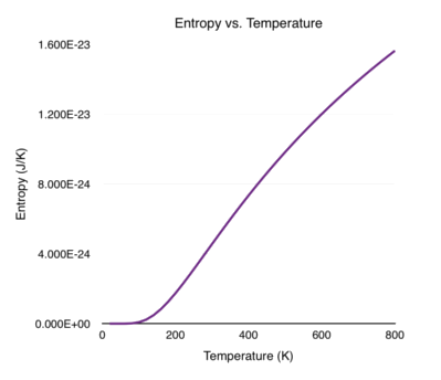
\[\begin{align} S &= -\frac{\partial}{\partial T} \left [ \frac{\hbar \omega}{2} + \frac{1}{\beta} ln \left ( 1 - e^{-\beta \hbar \omega} \right ) \right ]\\[0.1cm] &= -\frac{\partial}{\partial T} \left [ kT ln \left ( 1 - e^{-\hbar \omega/(kT)} \right ) \right ]\\[0.1cm] &= -k ln \left ( 1 - e^{-\hbar \omega/(kT)} \right ) - \left ( \frac{kT}{1 - e^{-\hbar \omega/(kT)}} \right ) \left ( -\frac{\hbar\omega}{kT^2} e^{-\hbar\omega/(kT)} \right )\\[0.1cm] &= -k ln \left ( 1 - e^{-\hbar \omega/(kT)} \right ) + \left ( \frac{\hbar\omega}{T} \right ) \left ( \frac{e^{-\hbar\omega/(kT)}}{1 - e^{-\hbar \omega/(kT)}} \right )\\[0.1cm] &= -k ln \left ( 1 - e^{-\beta \hbar \omega} \right ) + \left ( \frac{\hbar\omega}{T} \right ) \left ( \frac{e^{-\beta \hbar\omega}}{1 - e^{-\beta \hbar \omega}} \right ) \end{align}\]Shown below is a plot of the entropy versus temperature (T). I set \(\hbar \omega = 1 \times 10^{-20}\) J, corresponding to oscillations (\(\omega\)) in the infrared light frequency.
The Average Energy
Finally, we can calculate the average energy of the quantum harmonic oscillator.
\[\begin{equation} \langle E \rangle = -\frac{\partial ln(Z)}{\partial \beta} \end{equation}\]Plug the partition function into the formula above and work through the exponentials.
\[\begin{align} \langle E \rangle &= -\frac{\partial ln(Z)}{\partial \beta}\\[0.1cm] &= -\frac{\partial}{\partial \beta} \left [ ln \left ( \frac{1}{e^{\beta\hbar\omega/2} - e^{-\beta\hbar\omega/2}} \right ) \right ]\\[0.1cm] &= \frac{\partial}{\partial \beta} \left [ ln \left ( e^{\beta\hbar\omega/2} - e^{-\beta\hbar\omega/2} \right ) \right ]\\[0.1cm] &= \frac{\frac{\hbar\omega}{2} e^{\beta\hbar\omega/2} + \frac{\hbar\omega}{2} e^{-\beta\hbar\omega/2}}{e^{\beta\hbar\omega/2} - e^{-\beta\hbar\omega/2}}\\[0.1cm] &= \frac{\hbar\omega}{2} \frac{e^{\beta\hbar\omega/2} + e^{-\beta\hbar\omega/2}}{e^{\beta\hbar\omega/2} - e^{-\beta\hbar\omega/2}}\\[0.1cm] &= \frac{\hbar\omega}{2} \frac{1 + e^{-\beta\hbar\omega}}{1 - e^{-\beta\hbar\omega}} \end{align}\]We can simplify this problem further by adding and subtracting an exponential in the numerator.
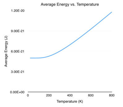
\[\begin{align} \langle E \rangle &= \frac{\hbar\omega}{2} \frac{1 + e^{-\beta\hbar\omega} + e^{-\beta\hbar\omega} - e^{-\beta\hbar\omega}}{1 - e^{-\beta\hbar\omega}}\\[0.1cm] &= \frac{\hbar\omega}{2} \frac{\left ( 1 - e^{-\beta\hbar\omega} \right ) + 2e^{-\beta\hbar\omega}}{1 - e^{-\beta\hbar\omega}}\\[0.1cm] &= \frac{\hbar\omega}{2} \frac{1 - e^{-\beta\hbar\omega}}{1 - e^{-\beta\hbar\omega}} + \frac{\hbar\omega}{2} \frac{2e^{-\beta\hbar\omega}}{1 - e^{-\beta\hbar\omega}}\\[0.1cm] &= \frac{\hbar\omega}{2} + \frac{\hbar\omega e^{-\beta\hbar\omega}}{1 - e^{-\beta\hbar\omega}} \end{align}\]The graph below shows the average energy of the system as a function of temperature. I set \(\hbar \omega = 1 \times 10^{-20}\) J, corresponding to oscillations (\(\omega\)) in the infrared light frequency.
Conclusions
And there we have it! We calculated and plotted some of the thermodynamic quantities corresponding to the quantum harmonic oscillator. Take a close look at the graphs for Helmholtz free energy and average energy. As the temperature approaches absolute zero, the energy does not go down to zero. Instead, it approaches \(\hbar \omega/2\). This is the famous zero-point energy that physicists love to talk about so much!
By the way, you might be wondering why I stopped with the thermodynamic quantities above. Why not calculate the chemical potential or the specific heat or any number of other quantities? Well, many of the other quantities only make sense if you have a collection of particles. With only one oscillator, chemical potential does not mean much.
Until next week!