The Molecular Zipper
Introduction
Physics students the world over encounter the zipper problem at some point in their studies. It is a simple statistical physics model of the formation or unraveling of a long chain of links (often used as a toy model for DNA). Part of the reason that the zipper problem is so popular in homework assignments is that it has a great balance of interesting physics with relatively simple calculations.
We can take this common homework problem a step further to uncover some new physics in the system. By adding a simple model of degeneracy to the links, we can actually uncover a phase transition in this seemingly innocent one-dimensional zipper. Let’s take a look.
The Setup
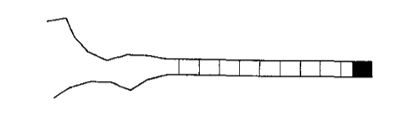
Suppose a zipper in a heat bath (temperature \(T\)) has \(N\) links. Each link can either be closed with energy 0 or open with energy \(\epsilon\). However, the zipper can only unzip from one end. Thus, link number \(s\) can only open if all links before it are also open (\(1, 2, \cdots, s - 1\)). Shown below is the zipper diagram in Kittel’s paper.
I am going to make a couple of assumptions here, just to simplify the analysis of the problem (similar to Kittel):
-
The final link can never be open (shown as a thick black square on the right side of the diagram above). This prevents the zipper from disconnecting and drifting apart.
-
When a link is closed it can only be in one configuration. However, when the link is open, the two pieces of the link are free to spin around and assume G different positions. Thus, the open link has a degeneracy of G.
The diagrams below show some possible examples of open links in different orientations. The orientation of the link does not change the energy stored in the link, so these setups all have the same total energy.

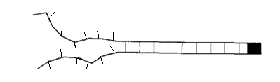
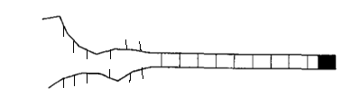
If I were to do this problem in a traditional statistical mechanics class, then \(G\) would be equal to one. However, if \(G\) is not equal to one, we see an interesting effect.
The Partition Function
Due to the restricted way that the chain of \(N\) links can unravel, it can only be in certain specific energy states. If the first \(s\) links are open, then the total energy of the system is equal to \(E_s = \epsilon s\). Let’s pretend that each of the links is some particle with energy 0 or \(\epsilon\). The links in the chain will never interact with each other - they just open or close if the conditions are right. If you have a system of non-interacting particles in thermal equilibrium, then you can use Maxwell-Boltzmann statistics.
The first step to solving any Maxwell-Boltzmann statistics problem is calculating the partition function. This is surprisingly easy for our single-ended zipper. Recall that a partition function is defined by the following sum:
\[\begin{equation} Z = \sum_{s=0}^M e^{-E_s/kT} \end{equation}\]In the expression above, \(s\) denotes a particular state, \(E_s\) is the energy of the state \(s\), \(k\) is Boltzman’s constant, and \(T\) is the temperature of the system. We are summing over the \(M\) possible states of the system. In the single-ended zipper problem, the different states correspond to different numbers of links being open (i.e. no links open, one link open, two links open, etc.). In each of these cases, we have a degeneracy \(G^s\) (i.e. there are \(G^s\) different ways that the open links can orient themselves, with each of those states having energy \(E_s = \epsilon\)s). Then:
\[\begin{equation} Z = \sum_{s=0}^{N-1} G^s e^{-E_s/kT} = \sum_{s=0}^{N-1} G^s e^{-s\epsilon/kT} = \sum_{s=0}^{N-1} \left [ G e^{-\epsilon/kT} \right ]^s \end{equation}\]In the equations above, we are summing to (N-1), not N. This is because we assume that the last link of the zipper will never be open (i.e. the two halves of the zipper can never disconnect and drift apart). Since \(\epsilon\), \(k\), and \(T\) are all positive, the exponent will always be less than or equal to one. Thus, we can turn to the geometric series to simplify the expression. Recall that:
\[\begin{equation} \sum_{a=0}^N r^a = \frac{1 - r^{N+1}}{1-r} \end{equation}\]Thus, our partition function can be re-written as:
\[\begin{equation} Z = \frac{1 - Ge^{-N\epsilon/kT}}{1 - Ge^{-\epsilon/kT}} \end{equation}\]As is customary in statistical mechanics, I will define \(\beta \equiv (kT)^{-1}\).
\[\begin{equation} Z = \frac{1 - Ge^{-\beta N\epsilon}}{1 - Ge^{-\beta \epsilon}} \end{equation}\]I am going to proceed similar to Kittel and define \(x \equiv Gexp(-\beta \epsilon)\). Then:
\[\begin{equation} Z = \frac{1 - x^N}{1 - x} \end{equation}\]
Average Number of Open Links
Once you determine the partition function, you can solve for any number of thermodynamic quantities. Traditionally, one is asked to solve for the average number of open links on the zipper \(\langle s \rangle\). This is just the sum over all states of the probability of being in that state (P) multiplied by the index of the state (s):
\[\begin{equation} \langle s \rangle = \sum_{s=0}^{N-1} sP(s) = \sum_{s=0}^{N-1} \frac{s e^{-\beta s \epsilon}}{Z} = \frac{1}{Z} \sum_{s=0}^{N-1} s e^{-\beta s \epsilon} \end{equation}\]Notice that we can rewrite the sum in terms of a derivative of the partition function (\(Z\)). The expression for \(\langle s \rangle\) becomes.
\[\begin{equation} \langle s \rangle = -\frac{1}{Z\epsilon} \frac{\partial Z}{\partial \beta} \end{equation}\]Now we utilize a common trick in thermodynamics calculations. Given a function \(f(\beta) \equiv f\):
\[\begin{equation} \frac{1}{f} \frac{\partial f}{\partial \beta} = \frac{\partial}{\partial \beta} ln(f) \end{equation}\]The expression for \(\langle s \rangle\) becomes:
\[\begin{equation} \langle s \rangle = -\frac{1}{\epsilon} \frac{\partial}{\partial \beta} ln(Z) \end{equation}\]This is pretty easy to simplify:
\[\begin{align} \langle s \rangle &= -\frac{1}{\epsilon} \frac{\partial}{\partial \beta} ln(Z)\\[0.1cm] &= -\frac{1}{\epsilon} \frac{\partial}{\partial \beta} ln \left (\frac{1-x^N}{1-x} \right )\\[0.1cm] &= -\frac{1}{\epsilon} \frac{\partial}{\partial \beta} \left [ ln(1-x^N) - ln(1-x) \right ]\\[0.1cm] &= -\frac{1}{\epsilon} \left [ \frac{\frac{\partial (1-x^N)}{\partial \beta}}{1-x^N} - \frac{\frac{\partial (1-x)}{\partial \beta}}{1-x} \right ] \end{align}\]Recall that \(x \equiv Gexp(-\beta \epsilon)\).
\[\begin{align} \langle s \rangle &= -\frac{1}{\epsilon} \left [ \frac{N\epsilon x^N}{1-x^N} - \frac{\epsilon x}{1-x} \right ]\\[0.1cm] &= \frac{Nx^N}{x^N - 1} - \frac{x}{x-1}\\[0.1cm] \end{align}\]Thus, we have arrived at a familiar answer.
The Phase Transition
The final expression above is the usual stopping point in most statistical mechanics classes. However, we are going to take it a step further. Take a look at the denominators in the expression above. Something interesting is happening in the liminting case when \(x\) approaches one. In the figures below, I plot the value of \(\langle s \rangle\) as a function of \(x\) at different values of \(N\). Notice that I center each graph around \(x = 1\).
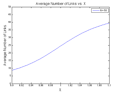
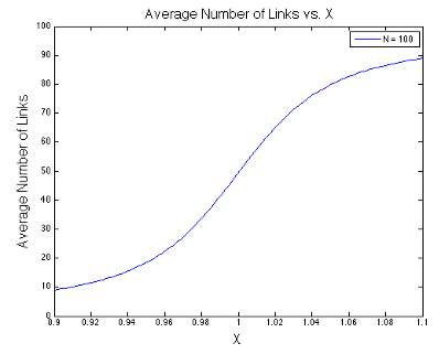
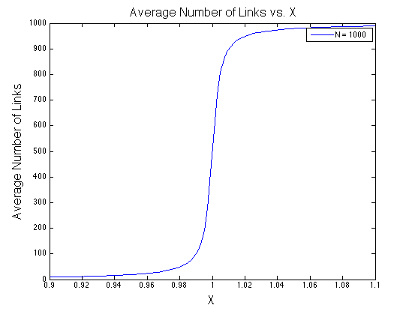
It looks like the expression has a discontinuity centered at \(x=1\) when \(N\rightarrow\infty\). This discontinuity corresponds to a phase change - the phase of relatively few links being open changes to the phase of almost all links being open.

Not quite little cupcake. It is true that \(exp(-\beta\epsilon)\) can never equal one, so we will never see a phase transition in the traditional solution to the zipper problem where \(G=1\). However, the expression \(x = Gexp(-\beta \epsilon)\) can equal one if G is large enough.
\[\begin{equation} Ge^{-\beta \epsilon} = 1 \end{equation}\] \[\begin{equation} G = e^{\beta \epsilon} \end{equation}\]When the degeneracy of the system is equal to \(exp(\beta\epsilon)\), we will see a phase transition. Pretty neat.
In the real world, we cannot control \(G\) or \(\epsilon\); they are fixed values for a given system. However, we can control the temperature of the heat bath \(T\). Thus, we can rearrange the equation above to get the temperature at which the phase transition occurs:
\[\begin{equation} G = e^{\beta \epsilon} = e^{\epsilon/kT} \end{equation}\] \[\begin{equation} ln(G) = \epsilon/kT \end{equation}\] \[\begin{equation} T = \frac{\epsilon}{k ln(G)} \end{equation}\]Pretty snazzy.