The Diffusion Equation (Part 2)
Introduction
Source code for this post can be found here.
In my post from a couple of weeks ago, I mentioned that there are two major ways that we normally use to get an analytical solution for the diffusion equation. You can use the method of separation of variables (which I might cover in a future post) or you can use the Laplace transform. We took the Laplace transform of the diffusion equation and went through a lot of math. At the end of the day, we got an interesting little expression for how a concentrated number of particles diffuses in a system.
\[\begin{equation} \phi(x,t) = \frac{1}{\sqrt{4\pi Dt}} e^{-x^2/(4Dt)} \end{equation}\]In the equation above, \(x\) is position in one dimension, \(D\) is the diffusivity coefficient, and \(t\) is time. Let’s take a moment to visualize this equation. Then, we can expand it to cover any arbitrary particle distribution.
Dirac Delta Function Number Density
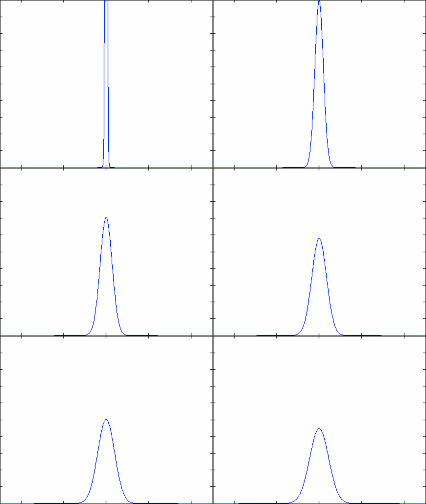
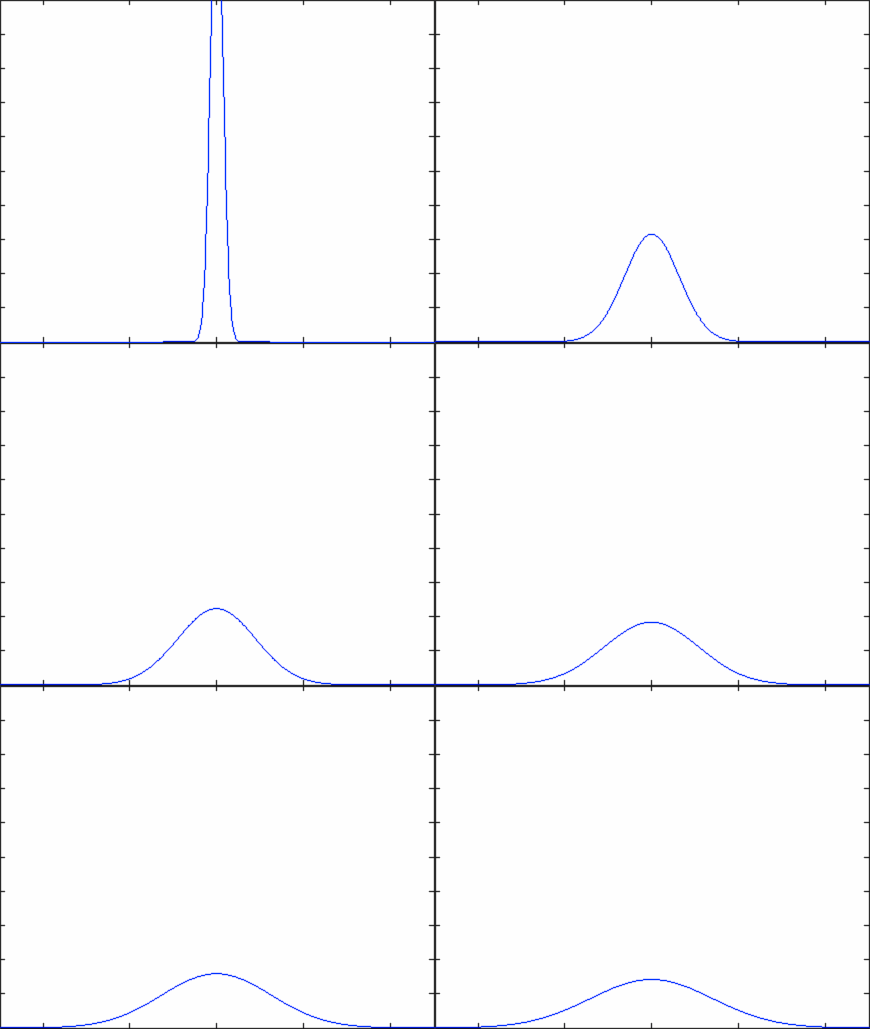
The equation above describes how an initial particle distribution that is concentrated at the origin would evolve as a function of time. Notice that at time \(t=0\), the concentration of particles follows a Dirac Delta function - the density of particle is zero everywhere except for the origin. At the origin itself, the density of particles is infinitely large due to the variable \(t\) in the denominator of the equation. As time evolves, the number density of particles is described by a normal distribution that grows ever wider - this means that the particles are spreading out in space, as we would expect.
Play around with the file called diffusion.m to see the evolution of a concentrated number density of particles as a function of time. Notice that I do not start the simulation exactly at time \(t=0\), but rather just slightly afterwards. This is just to keep the graphs looking nice (it is hard to plot infinity).
You can generate nice plots that show the number density of particles in a position vs. time:

Or you can crank up the diffusivity coefficient (D) and watch the particles really move!

In the graphs above, the horizontal axis is position while the vertical axis is particle number density. Everything is labeled nicely in the Matlab program (including axes).
Convolutions
A single Dirac Delta peak is fine, but we really need a way to visualize the diffusion of any arbitrary density of particles. For example, what if I dump a bunch of dye into a bucket of water? That is certainly not a single point of dye diffusing as a nice, neat Gaussian distribution. Let’s return to the derivation from last week and look at the third to the last line. I wrote the following expression:
\[\begin{equation} \phi(x,t) = \int_{-\infty}^\infty \frac{1}{\sqrt{4\pi Dt}} e^{-|x - \alpha|^2/(4Dt)} \phi(\alpha, 0) d\alpha \end{equation}\]Let’s begin our analysis of this expression by renaming one term within the integral. I am going to call the exponential term the heat kernel (it is studied a lot in heat transfer problems). It will be represented by:
\[\begin{equation} K(x-\alpha, t) = \frac{1}{\sqrt{4\pi Dt}} e^{-|x - \alpha|^2/(4Dt)} \end{equation}\]The heat kernel is a function of position (\(x - \alpha\)) and time (\(t\)). You might notice that it is simply the expression that we analyzed in the previous section. The only difference is that the extra \(\alpha\) in the expression simply shifts the bell curve left or right along the axis (as you can see in the following plot).
We can rewrite the integral as:
\[\begin{equation} \phi(x,t) = \int_{-\infty}^\infty K(x-\alpha, t) \phi(\alpha, 0) d\alpha \end{equation}\]This is interesting…
The integral itself is in terms of \(\alpha\); the time \(t\) is just along for the ride. The expression \(\phi(\alpha, 0)\) gives the number density at some position in space \(\alpha\) at the time \(t=0\). Let’s just fix the time \(t\) as a constant for a moment since it does not affect the actual integration. Then:
\[\begin{equation} \phi(x) = \int_{-\infty}^\infty K(x-\alpha) \phi(\alpha) d\alpha \end{equation}\]Anybody who has studied the theory behind signal processing might immediately recognize that formula. That is a convolution! A convolution basically tells you the amount of overlap between one function as you move it over another (take a look at the great animations on Wolfram Mathworld from the link above).
So what are we saying here? We know how a particle density concentrated on a single point would evolve in time (the example of the Dirac Delta function). So, if you want analyze any arbitrary particle density function, break it up into lots of little points, analyze each little point as if it were a Dirac Delta function, and then add all of those final analyses together. This can be done by using a convolution.
We can write the general expression for the number density of particles at any given position and any given time as a convolution:
\[\begin{equation} \phi(x,t) = K(x, t) \ast \phi(x, 0) \end{equation}\]Conclusion
Convolutions and kernels don’t often appear until more advanced physics classes, but the concept behind these seemingly complex mathematical strucutres is very simple. Since we cannot analyze all of space at once, we can cut it up into tiny pieces, analyze each piece individually, and then add all of the calculations back together.
Until next week!