Linear Interpolation
Linear Interpolation
Oftentimes in physics or engineering, we know the value of a quantity at certain points but not others. For example take a look at this saturation table for water. We know the thermodynamic properties of water at certain temperatures (\(5^\circ C\), \(10^\circ C\), \(15^\circ C\),…). However, suppose we want to know the saturation pressure of water at \(32^\circ C\). What do we do? It’s not on the table!

Linear interpolation allows us to figure out the values between entires in that table. It is easiest to think about linear interpolation in terms of the graph of a straight line. Take a look at the simple graph of a line below.
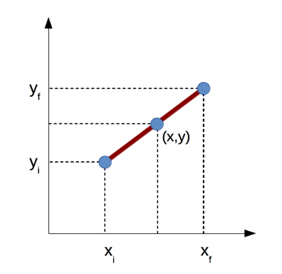
Suppose we know the values of two points on the graph: \((x_i,y_i)\) and \((x_f, y_f)\). We want to determine the value of \(y\) at some point \(x\) along the line connecting the two known points. First, we can write out a simple ratio that relates the known values to the unknown values.
\[\begin{equation} \frac{y - y_i}{x - x_i} = \frac{y_f - y_i}{x_f - x_i} \end{equation}\]Now, we can multiply each side of the expression by \((x - x_i)\).
\[\begin{equation} y - y_i = \frac{x - x_i}{x_f - x_i} \left ( y_f - y_i \right ) \end{equation}\]Finally, we can move \(y_i\) to the other side of the equation to get the formula for \(y\).
\[\begin{equation} y = y_i + \frac{x - x_i}{x_f - x_i} \left ( y_f - y_i \right ) \end{equation}\]Going back to the saturation table from before, suppose I want to determine the saturation pressure for water at \(32^\circ C\) (\(P_{32^\circ C}\)). We will let the \(y\) variables represent pressure and the \(x\) variables represent temperature. Plugging in the appropriate values gives:
\[\begin{equation} P_{32^\circ C} = P_{30^\circ C} + \frac{32^\circ C - 30^\circ C}{35^\circ C - 30^\circ C} \left ( P_{35^\circ C} - P_{30^\circ C} \right ) \end{equation}\] \[\begin{equation} P_{32^\circ C} = 4.2460 \hspace{1mm} kPa + \frac{2}{5} \left ( 5.6280 \hspace{1mm} kPa - 4.2460 \hspace{1mm} kPa \right ) \end{equation}\] \[\begin{equation} P_{32^\circ C} = 4.7988 \hspace{1mm} kPa \end{equation}\]Linear interpolation is not just restricted to table entires. Suppose I have some continuous function \(f(x)\). I can pick two points along the curve and estimate the value of the function at some point between them using the equation above. However, we have to be careful - our estimate may not be very accurate if the function \(f(x)\) is very curvy.
Visualizing the Error in Linear Interpolation
There are lots of websites that derive the error bounds in linear interpolation (e.g. here and here and here and here). Instead of doing yet another error derivation, I would like to visualize what linear interpolation is actually doing. From there, it is easy to see where the error comes from.
In the graph below, I have plotted an equation that has lots of bends and wiggles:
\[\begin{equation} f(x) = 2 cos(2x) + sin(6x) + 4 \end{equation}\]You can adjust the \(x\) values of the endpoints and the point of interpolation. The readout will tell you the percent error of the interpolated value (\(y\)) versus the actual value of the function at \(x\). Think about a couple of things as you play with the simulation:
- How does the error change as the known points get farther apart?
- How does the error change between the extra curvy parts of the graph and the straighter parts of the graph?
| Endpoint A | (0.00, 6.00) | |
| Endpoint B | (3.00, 5.17) | |
| Interpolated Point (C) | (1.50, 5.58) | |
| Percent Error | 129.62 % |