An Oscillating Electron Around a Ring of Charge (Part 3)
A Quick Review
It’s been a few weeks since we started this problem, but we are finally in the home stretch! Let’s go over some of the major equations that we ran into over the last couple of posts. First, we derived the electric field from a ring of charge using Coulomb’s law.
\[\begin{equation} E_z = \frac{k Q z} {\left (z^2 + R^2 \right )^{3/2}} \end{equation}\]We then analyzed the oscillatory motion of an electron in this electric field. Recall that we used the assumption that \(R \gg z\) in order to derive an analytic solution.
\[\begin{equation} \ddot{z} + \frac{k Qe }{mR^3}z = 0 \end{equation}\] \[\begin{equation} z(t) = Asin \left (\sqrt{\frac{k Qe }{mR^3}} t \right ) + Bcos \left (\sqrt{\frac{k Qe }{mR^3}} t \right ) \end{equation}\]The solution above does not take into account any sort of radiation from the accelerating electron. In order to fix that problem, we found an expression for the self force on a charged particle - the recoil force that it feels when it radiates energy.
\[\begin{equation} \vec{F}_{AL} = \frac{e^2}{6 \pi \epsilon_o c^3} \frac{d\vec{a}}{dt} \end{equation}\]Then, we included the self force in the differential equation for the motion of the electron. We noted that it was one of the few times that the jerk of a particle came into play.
\[\begin{equation} \dddot{z} - \left ( \frac{6 m \pi \epsilon_o c^3}{e^2} \right ) \ddot{z} - \left ( \frac{6 kQ \pi \epsilon_o c^3}{e} \right ) \left ( \frac{z}{\left [ z^2 + R^2 \right ]^{3/2}} \right ) = 0 \end{equation}\]It seems like we are ready to solve this differential equation. However, there is one last snaffoo that we will run into if we are not careful. Let’s take a look.
Our First Try
Suppose we try to solve the differential equation as it stands right now. It is a third order, non-linear differential equation; thus, it might be easiest to solve it using numerical methods. We can plug our equation into Matlab’s trusty ode45 function and turn the crank.
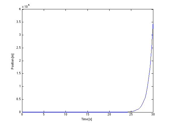

What on earth is going on? The position of the electron diverges instead of oscillating like we would expect.
The answer lies back in our derivation of the Abraham-Lorentz force. We assumed periodic motion of a point charge when deriving this force. In this specific example, as the electron radiates, the amplitude of its motion is going to shrink. Thus, this differential equation does not describe periodic motion, and the expression for self force that we derived cannot be used as is.
If we want to use our expression for self force, we need some way to force periodic motion on this system. One of the easiest ways to do this is to add a driving force that will ensure that the electron has periodic motion.
The Periodic Driver
Let’s change the problem slightly; we will enforce periodic motion on the electron by adding in a driving force with a frequency \(\omega\) and amplitude \(F_o\).
\[\begin{equation} F_{driving} = F_o cos(\omega t) \end{equation}\]Now, the differential equation describing the motion of the electron becomes:
\[\begin{equation} \vec{F}_{total} = \vec{F}_E + \vec{F}_{AL} + \vec{F}_{driving} \end{equation}\] \[\begin{equation} m \ddot{z} = - \frac{kQez}{\left [ z^2 + R^2 \right ]^{3/2}} + \frac{e^2}{6 \pi \epsilon_o c^3} \dddot{z} + F_o cos(\omega t) \end{equation}\]The electron will be forced to oscillate with a frequency of \(\omega\) due to \(F_{driving}\). This is great for us - we can assume a sinusoidal solution with an amplitude of \(z_o\), a frequency of \(\omega\), and a phase delay of \(\delta\).
\[\begin{equation} z(t) = z_o cos(\omega t - \delta) \end{equation}\]Let’s take time derivatives of this solution so that we can plug them back into the differential equation above.
\[\begin{equation} z = z_o cos(\omega t - \delta) \end{equation}\] \[\begin{equation} \dot{z} = -\omega z_o sin(\omega t - \delta) \end{equation}\] \[\begin{equation} \ddot{z} = -\omega^2 z_o cos(\omega t - \delta) \end{equation}\] \[\begin{equation} \dddot{z} = \omega^3 z_o cos(\omega t - \delta) = -\omega^2 \dot{z} \end{equation}\]Notice how the third derivative of position can be rewritten in terms of the first derivative of position. Thus, we can rewrite the third order differential equation as a second order differential equation.
\[\begin{equation} m \ddot{z} = - \frac{kQez}{\left [ z^2 + R^2 \right ]^{3/2}} - \frac{e^2 \omega^2}{6 \pi \epsilon_o c^3} \dot{z} + F_o cos(\omega t) \end{equation}\] \[\begin{equation} m \ddot{z} + \frac{kQez}{\left [ z^2 + R^2 \right ]^{3/2}} + \frac{e^2 \omega^2}{6 \pi \epsilon_o c^3} \dot{z} = F_o cos(\omega t) \end{equation}\]At this point we could solve the equation numerically using Matlab or some other program. However, let’s try to get an analytic solution to this problem so that we can really get a sense of its motion. Like we did before, take the limit of \(R \gg z\).
\[\begin{equation} m \ddot{z} + \frac{e^2 \omega^2}{6 \pi \epsilon_o c^3} \dot{z} + \frac{kQe}{R^3} z = F_o cos(\omega t) \end{equation}\] \[\begin{equation} \ddot{z} + \frac{e^2 \omega^2}{6 \pi \epsilon_o m c^3} \dot{z} + \frac{kQe}{mR^3} z = \frac{F_o}{m} cos(\omega t) \end{equation}\]That’s interesting. The coefficient in front of z is exactly the frequency we calculated in the case with no driving force and no radiation reaction. Just to keep our notation clear, we will call this the natural frequency of the system (\(\omega_o^2 = kQe/mR^3\)). Additionally, we will call the coefficient in front of \(\dot{z}\) the damping coefficient of the system (\(\gamma\)). Thus, we can rewrite the differential equation in a compact form.
\[\begin{equation} \ddot{z} + \gamma \dot{z} + \omega_o^2 z = \frac{F_o}{m} cos(\omega t) \end{equation}\]
So it is! Let’s go through the solution of this equation. Anybody who has taken an intermediate mechanics course should be very familiar with this solution. First, I will plug in the expressions for \(z\), \(\dot{z}\), and \(\ddot{z}\).
\[\begin{equation} -\omega^2 z_o cos(\omega t - \delta) - \gamma \omega z_o sin(\omega t - \delta) + \omega_o^2 z_o cos(\omega t - \delta) = \frac{F_o}{m} cos(\omega t) \end{equation}\] \[\begin{equation} \left ( \omega_o^2 - \omega^2 \right ) z_o cos(\omega t - \delta) - \gamma \omega z_o sin(\omega t - \delta) = \frac{F_o}{m} cos(\omega t) \end{equation}\]We can simplify this expression further. I refer to this table of trig identities to break up the sine and cosine terms.
\[\begin{equation} \left ( \omega_o^2 - \omega^2 \right ) z_o \left [ cos(\omega t)cos(\delta) + sin(\omega t)sin(\delta) \right ] - \gamma \omega z_o \left [ sin(\omega t)cos(\delta) - cos(\omega t)sin(\delta) \right ] = \frac{F_o}{m} cos(\omega t) \end{equation}\] \[\begin{equation} \left [ \left ( \omega_o^2 - \omega^2 \right ) z_o cos(\delta) + \gamma \omega z_o sin(\delta) - \frac{F_o}{m} \right ] cos(\omega t) + \left [ \left ( \omega_o^2 - \omega^2 \right ) z_o sin(\delta) - \gamma \omega z_o cos(\delta) \right ] sin(\omega t) = 0 \end{equation}\]In order for the equation above to equal zero, the sine and cosine pieces of the expression must each equal zero separately since they are orthogonal functions. We will start with the sine expression and solve for the phase (\(\delta\)).
\[\begin{align} \left [ \left ( \omega_o^2 - \omega^2 \right ) z_o sin(\delta) - \gamma \omega z_o cos(\delta) \right ] sin(\omega t) &= 0\\[0.1cm] \left ( \omega_o^2 - \omega^2 \right ) z_o sin(\delta) - \gamma \omega z_o cos(\delta) &= 0\\[0.1cm] \left ( \omega_o^2 - \omega^2 \right ) sin(\delta) - \gamma \omega cos(\delta) &= 0\\[0.1cm] \end{align}\] \[\begin{align} \left ( \omega_o^2 - \omega^2 \right ) sin(\delta) &= \gamma \omega cos(\delta)\\[0.1cm] tan(\delta) &= \frac{\gamma \omega}{\omega_o^2 - \omega^2}\\[0.1cm] \delta &= tan^{-1} \left ( \frac{\gamma \omega}{\omega_o^2 - \omega^2} \right ) \end{align}\]We can now analyze the cosine term in the expression to solve for the amplitude \(z_o\).
\[\begin{align} \left [ \left ( \omega_o^2 - \omega^2 \right ) z_o cos(\delta) + \gamma \omega z_o sin(\delta) - \frac{F_o}{m} \right ] cos(\omega t) &= 0\\[0.1cm] \left ( \omega_o^2 - \omega^2 \right ) z_o cos(\delta) + \gamma \omega z_o sin(\delta) - \frac{F_o}{m} &= 0 \end{align}\]We can rewrite the sine and cosine functions in terms of tangent in order to eliminate the dependence on \(\delta\). The cosine function becomes:
\[\begin{align} cos(\delta) &= \frac{1}{\sqrt{1 + tan^2(\delta)}}\\[0.1cm] &= \frac{1}{\sqrt{1 + \left ( \frac{\gamma \omega}{\omega_o^2 - \omega^2} \right )^2}}\\[0.1cm] &= \frac{1}{\sqrt{\frac{\left ( \omega_o^2 - \omega^2 \right )^2}{\left ( \omega_o^2 - \omega^2 \right )^2} + \frac{ \left ( \gamma \omega \right )^2}{ \left ( \omega_o^2 - \omega^2 \right )^2}}}\\[0.1cm] &= \frac{1}{\sqrt{\frac{\left ( \omega_o^2 - \omega^2 \right )^2 + \left ( \gamma \omega \right )^2}{\left ( \omega_o^2 - \omega^2 \right )^2}}}\\[0.1cm] &= \sqrt{\frac{\left ( \omega_o^2 - \omega^2 \right )^2}{\left ( \omega_o^2 - \omega^2 \right )^2 + \left ( \gamma \omega \right )^2}}\\[0.1cm] &= \frac{\omega_o^2 - \omega^2}{\sqrt{\left ( \omega_o^2 - \omega^2 \right )^2 + \left ( \gamma \omega \right )^2}}\\[0.1cm] \end{align}\]And the sine function becomes:
\[\begin{align} sin(\delta) &= \frac{tan(\delta)}{\sqrt{1 + tan^2(\delta)}}\\[0.1cm] &= \frac{\frac{\gamma \omega}{\omega_o^2 - \omega^2}}{\sqrt{1 + \left ( \frac{\gamma \omega}{\omega_o^2 - \omega^2} \right )^2}}\\[0.1cm] &= \frac{\frac{\gamma \omega}{\omega_o^2 - \omega^2}}{\sqrt{\frac{\left ( \omega_o^2 - \omega^2 \right )^2}{\left ( \omega_o^2 - \omega^2 \right )^2} + \frac{ \left ( \gamma \omega \right )^2}{ \left ( \omega_o^2 - \omega^2 \right )^2}}}\\[0.1cm] &= \frac{\frac{\gamma \omega}{\omega_o^2 - \omega^2}}{\sqrt{\frac{\left ( \omega_o^2 - \omega^2 \right )^2 + \left ( \gamma \omega \right )^2}{\left ( \omega_o^2 - \omega^2 \right )^2}}}\\[0.1cm] &= \frac{\gamma \omega}{\omega_o^2 - \omega^2} \sqrt{\frac{\left ( \omega_o^2 - \omega^2 \right )^2}{\left ( \omega_o^2 - \omega^2 \right )^2 + \left ( \gamma \omega \right )^2}}\\[0.1cm] &= \frac{\gamma \omega}{\sqrt{\left ( \omega_o^2 - \omega^2 \right )^2 + \left ( \gamma \omega \right )^2}}\\[0.1cm] \end{align}\]Let’s plug these expressions for sine and cosine into our original expression.
\[\begin{align} \left ( \omega_o^2 - \omega^2 \right ) z_o cos(\delta) + \gamma \omega z_o sin(\delta) - \frac{F_o}{m} &= 0\\[0.1cm] \frac{z_o \left (\omega_o^2 - \omega^2 \right )^2}{\sqrt{\left ( \omega_o^2 - \omega^2 \right )^2 + \left ( \gamma \omega \right )^2}} + \frac{z_o \left ( \gamma \omega \right )^2}{\sqrt{\left ( \omega_o^2 - \omega^2 \right )^2 + \left ( \gamma \omega \right )^2}} - \frac{F_o}{m} &= 0\\[0.1cm] z_o \left [ \frac{\left (\omega_o^2 - \omega^2 \right )^2}{\sqrt{\left ( \omega_o^2 - \omega^2 \right )^2 + \left ( \gamma \omega \right )^2}} + \frac{\left ( \gamma \omega \right )^2}{\sqrt{\left ( \omega_o^2 - \omega^2 \right )^2 + \left ( \gamma \omega \right )^2}} \right ] &= \frac{F_o}{m} \end{align}\] \[\begin{equation} z_o \left [ \frac{\left (\omega_o^2 - \omega^2 \right )^2 + \left ( \gamma \omega \right )^2}{\sqrt{\left ( \omega_o^2 - \omega^2 \right )^2 + \left ( \gamma \omega \right )^2}} \right ] = \frac{F_o}{m} \end{equation}\] \[\begin{equation} z_o \sqrt{\left ( \omega_o^2 - \omega^2 \right )^2 + \left ( \gamma \omega \right )^2} = \frac{F_o}{m} \end{equation}\] \[\begin{equation} z_o = \frac{F_o/m}{\sqrt{\left ( \omega_o^2 - \omega^2 \right )^2 + \left ( \gamma \omega \right )^2}}\\[0.1cm] \end{equation}\]Alright, let’s put everything together and get our final answer!
\[\begin{align} z(t) &= z_o cos(\omega t - \delta)\\[0.1cm] &= \frac{F_o/m}{\sqrt{\left ( \omega_o^2 - \omega^2 \right )^2 + \left ( \gamma \omega \right )^2}} cos \left ( \omega t - \delta \right )\\[0.1cm] &= \frac{F_o/m}{\sqrt{\left ( \frac{k Qe }{mR^3} - \omega^2 \right )^2 + \left ( \frac{e^2 \omega^3}{6 \pi \epsilon_o m c^3} \right )^2}} cos \left [ \omega t - tan^{-1} \left ( \frac{\frac{e^2 \omega^3}{6 \pi \epsilon_o m c^3}}{\frac{kQe}{mR^3} - \omega^2} \right ) \right ] \end{align}\] \[\begin{equation} z(t) = \frac{F_o/m}{\sqrt{\left ( \frac{k Qe }{mR^3} - \omega^2 \right )^2 + \left ( \frac{e^2 \omega^3}{6 \pi \epsilon_o m c^3} \right )^2}} cos \left [ \omega t - tan^{-1} \left ( \frac{e^2 \omega^3 R^3}{6 \pi \epsilon_o c^3 \left ( kQe - m \omega^2 R^3 \right )} \right ) \right ] \end{equation}\]Conclusions
This has been a pretty intense arc. We started off with an introductory physics problem - finding the electric field due to a ring of charge and the equation of motion for an electron oscillating about its center. Then, we stepped it up by adding the radiation reaction force to the mix. We were careful to enforce periodic motion on the electron so that the answer did not diverge. After all that, we saw that the equation of motion for the electron was exactly that of a damped, driven harmonic oscillator.
Take some time to go through each of the three posts in this arc. They describe a classic way to analyze problems in physics - start off with a simple model and then add layers of complexity to it when they are needed.