An Oscillating Electron Around a Ring of Charge (Part 1)
Introduction
This week in class, my students were trying their hand at solving for the electric potential and electric field from continuous charge distributions. It was the first time that many of them actually applied integrals to a physical setup. In the spirit of continuous charge distributions, I want to go over an example that was done in class and take it a step further.
First, I will derive the equation for the electric field along the axis of a ring of charge. Then, I will take the limit of the ring radius being much greater than the position along the axis. Finally, I will use that result to calculate the equation of motion for an electron released near the center of the ring.
Electric Field Along the Axis of a Charged Ring
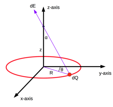
This derivation can be found all over the internet. I will quickly go through it here, just to set up the problem. Suppose I have a ring with total charge \(Q\) and radius \(R\). I want to find the electric field at some distance \(z\) along the z-axis as shown in the diagram below.
We can start by writing out Coulomb’s law for continuous charge distributions.
\[\begin{equation} d\vec{E} = \frac{k dQ}{r^2} \hat{r} \end{equation}\]Let’s start by solving for dQ in the equation above. As shown in the diagram, we cut the ring up into tiny little pieces. Each piece has a tiny charge dQ. If we define the charge density of the ring as \(\lambda = Q/2\pi R\) - the total charge of the ring divided by the total circumference of the ring - we can rewrite dQ in terms of charge density (\(\lambda\)) and arc length (\(ds\)).
\[\begin{equation} dQ = \lambda ds \end{equation}\]I personally like to integrate with respect to angle \(\theta\) rather than arc length. Thus, we can use the relationship between angle (\(d\theta\)) and arc length (\(ds\)) to expand the equation above.
\[\begin{equation} ds = R d\theta \end{equation}\] \[\begin{equation} dQ = \lambda R d\theta \end{equation}\]Next, we can solve for \(r^2\). This is particularly easy in this example - every tiny piece \(dQ\) along the ring is equidistant from the point some distance along the z-axis. We can calculate this distance using the Pythagorean theorem.
\[\begin{equation} r^2 = z^2 + R^2 \end{equation}\]Finally, we can solve for the unit vector \(\hat{r}\). In this case, we notice that all of the horizontal components of the electric field will cancel out, leaving only the vertical componenets. Thus, we can use the cosine function to get just the vertical component of the field.
\[\begin{equation} \hat{r} = cos\alpha \hat{z} \end{equation}\]We can rewrite the cosine in terms of z and R.
\[\begin{equation} cos\alpha \hat{z} = \frac{z}{r} \hat{z} = \frac{z}{\sqrt{R^2 + z^2}} \hat{z} \end{equation}\]Putting everything together gives us an expression for \(dE\) (now called \(dE_z\) to signify that the field points along the z-axis).
\[\begin{equation} dE_z = \frac{k z \lambda R d\theta}{\left (z^2 + R^2 \right )^{3/2}} \end{equation}\]I am will integrate this expression over the entire ring (angle 0 to \(2\pi\)).
\[\begin{align} E_z &= \int_0^{2\pi} \frac{k z \lambda R d\theta}{\left (z^2 + R^2 \right )^{3/2}}\\[0.1cm] &= \frac{k z \lambda R}{\left (z^2 + R^2 \right )^{3/2}} \int_0^{2\pi} d\theta\\[0.1cm] &= \frac{k z \lambda R}{\left (z^2 + R^2 \right )^{3/2}} \left ( 2\pi \right ) \end{align}\]We can simplify the charge density with the circumference (\(2\pi R\)) to get the final answer.
\[\begin{equation} E_z = \frac{k Q z} {\left (z^2 + R^2 \right )^{3/2}} \end{equation}\]Small Distance (z)
Suppose we are only interested in the electric field very close to the center of the ring. In other words, \(R \gg z\). Then, the \(R^2\) term in the denominator would completely dwarf the \(z^2\) term in the denominator. Thus, we can simplify the expression further for small distances (small z) by dropping \(z\) in the denominator.
\[\begin{equation} E_z \approx \frac{k Q z} {\left (0 + R^2 \right )^{3/2}} \end{equation}\] \[\begin{equation} E_z \approx \frac{k Q z} {R^3} \end{equation}\]Notice how this expression in linear with respect to \(z\) since \(k\), \(Q\), and \(R\) are all constants.
Oscillations About the Center of the Ring
An electron that is released very close to the center of a positively charged ring (along the z-axis) will feel a restoring force that we described above. Thus, it will oscillate about the center of the ring. We can actually calculate the frequency at which it oscillates. Start with Newton’s second law:
\[\begin{equation} \vec{F} = m\vec{a} \end{equation}\]In this case, the force \(\vec{F}\) is the force of the ring on the electron (i.e. the field \(E_z\) multiplied by the charge of an electron \(e\)). I will write the acceleration \(\vec{a}\) using dot notation (\(\ddot{z}\)).
\[\begin{equation} -\frac{k Qe }{R^3}z = m \ddot{z} \end{equation}\] \[\begin{equation} m \ddot{z} + \frac{k Qe }{R^3}z = 0 \end{equation}\] \[\begin{equation} \ddot{z} + \frac{k Qe }{mR^3}z = 0 \end{equation}\]As we expect, this is simply the equation for oscillatory motion! We can let \(\omega^2 = kQe/mR^3\) to see it more clearly.
\[\begin{equation} \ddot{z} + \omega^2 z = 0 \end{equation}\]The solution to this differential equation is our well known sum of a sine and cosine.
\[\begin{equation} z(t) = Asin(\omega t) + Bcos(\omega t) \end{equation}\] \[\begin{equation} z(t) = Asin \left (\sqrt{\frac{k Qe }{mR^3}} t \right ) + Bcos \left (\sqrt{\frac{k Qe }{mR^3}} t \right ) \end{equation}\]Conclusion
It’s nice to see the formula for oscillatory motion pop up again in introductory electromagnetism. It means that all of the stuff that we learned in mechanics is still valid! Next week, we will look a bit deeper at how to improve this equation of motion by taking into account the self-force - the force that an accelerating charge feels due to the fact that it radiates.
Until next week!