###Background

The Larmor formula is a neat little expression that is used to calculate the total power radiated by an accelerating point charge in the non-relativistic regime. I have seen this formula derived in a couple of different ways: first using Maxwell’s equations coupled with advanced/retarded potentials (Griffiths Chapter 11) and second using the Lienard-Wiechert potential (Jackson Chapter 9). Yes, to be fair, these are almost the same method; we just like to use the term “Lienard-Wiechert potential” in graduate school in order to impress people.

Yesterday, I had the pleasure of meeting up for coffee with one of my students. He showed me a simple geometric arguement for deriving the Larmor equation that was first introduced by J.J. Thomson. A description of the Thomson derivation can be found in many online sources and in Purcell’s book.

When I looked at some of the resources online, I found that a lot of instructors posted slightly abridged diagrams with their derivations. This can make it difficult to see where each variable comes from. I am going to go through the derivation in detail, refering to Purcell’s original diagram in Appendix B of his book. And Chaitanya, if you are reading this, thanks for the idea for the post!

###Purcell’s Diagram

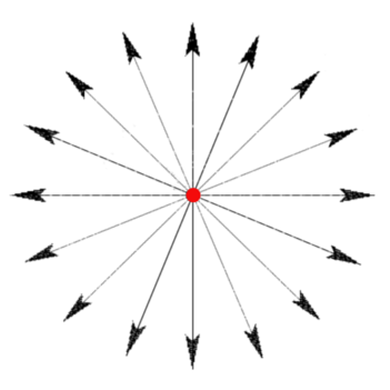
Consider a point charge q at rest. The electric field lines from the point charge have a simple radial configuration shown in the figure below.

Now suppose that the point charge initially moves in the \(+\hat{x}\)-direction with a speed of \(v_o\). When it passes the origin of our coordinate system, it decelerates to a halt over a short amount of time \(\tau\). We then measure the electric field lines at some time \(T\) in the future where \(T \gg \tau\).

We can visualize the shape of the electric field lines using the diagram below:

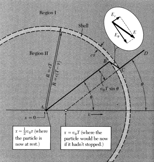
Let’s go through this picture in a bit more detail. The speed of light in a vacuum is the universal “speed limit”. No information can travel faster than the speed of light. Thus, the electric field lines cannot instantly change in all regions of space - instead, the information about the acceleration of the particle propagates through these field lines with speed c.

The expression \(R = cT\) is the distance that a pulse of light would travel from the origin in a time \(T\). The expression \(R = c(T-\tau)\) is the distance that a pulse of light would travel when the particle moves from the origin to point A and then emits light. Notice that the difference between these two pulses creates a tiny shell in space. This shell divides space into two regions.

In Region I the electric field lines have not yet recieved the information about the deceleration, so they will look as if the particle is still traveling with speed \(v_o\) and nothing has changed. However, the field lines in Region II have received the information that the particle has decelerated, so they will match up to the final position of the particle (point A). The position of point A comes from kinematics. Solving for the acceleration yields:

\[\begin{align} \vec{v}_f &= \vec{v}_i + \vec{a}t\\[0.1cm] 0 &= v_o \hat{x} + \vec{a}\tau\\[0.1cm] \vec{a} &= -\frac{v_o}{\tau} \hat{x} \end{align}\]

And then using that to find the final position:

\[\begin{align} \vec{x}_f &= \vec{x}_i + \vec{v}_i t + \frac{1}{2}\vec{a}t^2\\[0.1cm] &= 0 + v_o \tau \hat{x} - \frac{1}{2}\frac{v_o}{\tau}\tau^2 \hat{x}\\[0.1cm] &= v_o t \hat{x} - \frac{1}{2}v_o \tau \hat{x}\\[0.1cm] &= \frac{1}{2}v_o \tau \hat{x}\\[0.1cm] \end{align}\]

The angle between AB and the x-axis is the same as the angle between CD and the x-axis - let’s call it \(\theta\). Since the particle would have traveled to a final position \(x = v_o T\) had it not decelerated, the perpendicular distance between AB and CD is \(v_oT sin\theta\).

The electric field lines need to be continuous, so their final shape is given by the series of segmets ABCD. This “kink” in the field lines is the electromagnetic wave that propagates through space.

We can find the radial and angular components of the “kink” in the field. The radial component of the electric field simply comes from Coulomb’s law:

\[\begin{equation} E_r = \frac{kq}{R^2} \approx \left ( \frac{1}{cT} \right ) \frac{kq}{R} \end{equation}\]

I expanded the expression using \(R = cT\) just to make future math a bit easier. Remember, \(T \gg \tau\), so \((T - \tau) \approx T\). The angular component of the electric field can be found using the ratio of the two electric field components. These components are proportional to the lengths that we calculated in the diagram above:

\[\begin{align} \frac{E_\theta}{E_r} &= \frac{v_o T sin\theta}{c\tau}\\[0.1cm] &= \frac{\frac{v_o}{\tau} T sin\theta}{c}\\[0.1cm] &= \frac{|a| T sin\theta}{c} \end{align}\]

Then:

\[\begin{align} E_\theta &= \left [ \frac{|a| Tsin\theta}{c} \right ] E_r\\[0.1cm] &= \left [ \frac{|a| Tsin\theta}{c} \right ] \left [ \frac{1}{cT} \frac{kq}{R} \right ]\\[0.1cm] &= \frac{kq|a| sin\theta}{c^2 R}\\[0.1cm] \end{align}\]

###The Larmor Formula

Now that we have \(E_\theta\), the derivation of the Larmor formula is straightforward. First, we can use the angular electric field to find the Poynting vector around the point charge:

\[\begin{align} |\vec{S}| &= \frac{1}{\mu_o} \left | \vec{E} \times \vec{B} \right |\\[0.1cm] &= \frac{1}{\mu_o} \left | |\vec{E}| |\vec{B}| sin(90^\circ) \right | \\[0.1cm] &= \frac{1}{\mu_o} \left ( EB \right )\\[0.1cm] &= \frac{1}{\mu_o} \left ( \frac{E^2}{c} \right )\\[0.1cm] &= \epsilon_o c E^2\\[0.1cm] &= \epsilon_o c \left [ \frac{kq|a| sin\theta}{c^2 R} \right ]^2\\[0.1cm] &= \frac{\epsilon_o k^2 q^2 a^2 sin^2\theta}{c^3 R^2}\\[0.1cm] \end{align}\]

We can integrate this expression over all angles in order to get the total power dissipated:

\[\begin{align} P &= \int |\vec{S}| R^2 d\Omega\\[0.1cm] &= \int_0^{2\pi} \int_0^\pi |\vec{S}| R^2 sin\theta d\theta d\phi\\[0.1cm] &= \int_0^{2\pi} \int_0^\pi \frac{\epsilon_o k^2 q^2 a^2 sin^2\theta}{c^3 R^2} R^2 sin\theta d\theta d\phi\\[0.1cm] &= \frac{\epsilon_o k^2 q^2 a^2}{c^3} \int_0^{2\pi} \int_0^\pi sin^3\theta d\theta d\phi\\[0.1cm] &= \frac{2\pi \epsilon_o k^2 q^2 a^2}{c^3} \int_0^\pi sin^3\theta d\theta\\[0.1cm] &= \frac{8\pi \epsilon_o k^2 q^2 a^2}{3c^3}\\[0.1cm] \end{align}\]

Expanding \(k = (4\pi\epsilon_o)^{-1}\) yields:

\[\begin{equation} P = \frac{8\pi \epsilon_o q^2 a^2}{48 \pi^2 \epsilon_o^2 c^3} \end{equation}\] \[\begin{equation} P = \frac{q^2 a^2}{6 \pi \epsilon_o c^3} \end{equation}\]

Thus, we have an expression for the power dissipated by a particle as it accelerates.