Small Angle Oscillations of the Double Pendulum
Background
When physicists study the double pendulum, they often do so in the context of chaos theory. It is one of the simplest dynamical systems that has chaotic solutions. However, under the right conditions, even the double pendulum simplifies down to a simple series of oscillators with well-defined normal modes.
Most derivations of the normal modes that I see online use Lagrangians or Hamiltonians to get to the final answer. These derivations are great, but we can also solve for the modes of the double pendulum using Newton’s laws. Let’s take a look.
The Double Pendulum
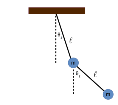
We will start off with a diagram of the double pendulum. Suppose two point masses (each with mass \(m\)) are attached to two massless strings (each with length \(\ell\)). We measure the angles \(\theta_1\) and \(\theta_2\) from the rest positions of each pendulum.
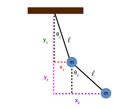
We can calculate the \(x\) and \(y\) positions of each mass using some simple trigonometry. Let \(x_1\) and \(y_1\) be the \(x\) and \(y\) positions of the upper mass. Let \(x_2\) and \(y_2\) be the \(x\) and \(y\) positions of the lower mass. We will set the origin of the system to be the point where the double pendulum is connected to the ceiling.
We want to analyze the motion of the double pendulum under small angle oscillations (\(\theta_1\) and \(\theta_2\) close to zero). In that case, we know that \(sin\theta \approx \theta\) and \(cos\theta \approx 1\).
\[\begin{equation} x_1 \approx \ell \theta_1 \Rightarrow \theta_1 \approx \frac{x_1}{\ell} \end{equation}\] \[\begin{equation} y_1 \approx - \ell \end{equation}\] \[\begin{equation} x_2 \approx \ell \left ( \theta_1 + \theta_2 \right ) \Rightarrow \theta_2 \approx \frac{x_2 - x_1}{\ell} \end{equation}\] \[\begin{equation} y_2 \approx -2 \ell \end{equation}\]Notice how \(y_1\) and \(y_2\) are constant under the small angle approximation - the masses have a tiny movement horizontally and have negligible motion in the vertical direction. Thus, we can ignore the \(y\)-component of acceleration. Let’s set up Newton’s laws for each mass along the horizontal (\(x\)) direction. Let \(T_1\) and \(T_2\) be the tensions in the upper and lower strings respectively.
\[\begin{align} m \ddot{x}_1 &= -T_1 sin\theta_1 + T_2 sin\theta_2\\[0.1cm] &\approx -T_1 \theta_1 + T_2 \theta_2\\[0.1cm] &\approx -T_1 \frac{x_1}{\ell} + T_2 \frac{x_2 - x_1}{\ell} \end{align}\] \[\begin{align} m \ddot{x}_2 &= -T_2 sin\theta_2\\[0.1cm] &\approx -T_2 \theta_2\\[0.1cm] &\approx -T_2 \frac{x_2 - x_1}{\ell} \end{align}\]The small angle approximation implies that the double pendulum will hang almost vertically, even during the oscillations. Thus, the magnitude of the tension in each string is simply equal to the weight of the masses that it supports; the tensions are \(T_1 \approx 2mg\) and \(T_2 \approx mg\).
Solving for \(\ddot{x}_1\) yields:
\[\begin{equation} m \ddot{x}_1 = -2mg \frac{x_1}{\ell} + mg \frac{x_2 - x_1}{\ell} \end{equation}\] \[\begin{align} \ddot{x}_1 &= \frac{g}{\ell} \left [ -2 x_1 + x_2 - x_1 \right ]\\[0.1cm] &= \frac{g}{\ell} \left [ -3 x_1 + x_2 \right ] \end{align}\]Solving for \(\ddot{x}_2\) yields:
\[\begin{equation} m \ddot{x}_2 = -T_2 \frac{x_2 - x_1}{\ell} \end{equation}\] \[\begin{equation} m \ddot{x}_2 = -mg \frac{x_2 - x_1}{\ell} \end{equation}\] \[\begin{align} \ddot{x}_2 = -\frac{g}{\ell} \left ( x_2 - x_1 \right ) \end{align}\]Let \(\omega_o \equiv \sqrt{g/\ell}\). Then:
\[\begin{equation} \ddot{x}_1 + 3\omega_o^2 x_1 - \omega_o^2 x_2 = 0 \end{equation}\] \[\begin{equation} \ddot{x}_2 + \omega_o^2 x_2 - \omega_o^2 x_1 = 0 \end{equation}\]It is easiest to solve this system of equations by writing it out in matrix form.
\[\begin{equation} \begin{bmatrix} \ddot{x}_1\\[0.1cm] \ddot{x}_2 \end{bmatrix} + \begin{bmatrix} 3\omega_o^2 & -\omega_o^2\\[0.1cm] -\omega_o^2 & \omega_o^2 \end{bmatrix} \begin{bmatrix} x_1\\[0.1cm] x_2 \end{bmatrix} = 0 \end{equation}\]Let’s assume that the oscillations have a form \(x(t) = C cos(\omega t + \delta)\) where \(C\) and \(\delta\) are constants. Then we can write out \(x_1(t)\) in the same form:
\[\begin{equation} x_1(t) = c_1 cos(\omega t + \delta_1) \end{equation}\] \[\begin{equation} \dot{x}_1(t) = -\omega c_1 sin(\omega t + \delta_1) \end{equation}\] \[\begin{equation} \ddot{x}_1(t) = -\omega^2 c_1 cos(\omega t + \delta_1) = -\omega^2 x_1 \end{equation}\]And we can do the same for \(x_2(t)\):
\[\begin{equation} x_2(t) = c_2 cos(\omega t + \delta_2) \end{equation}\] \[\begin{equation} \dot{x}_2(t) = -\omega c_2 sin(\omega t + \delta_2) \end{equation}\] \[\begin{equation} \ddot{x}_2(t) = -\omega^2 c_2 cos(\omega t + \delta_2) = -\omega^2 x_2 \end{equation}\]Plugging these expressions into the matrix equation yields:
\[\begin{equation} \begin{bmatrix} -\omega^2 x_1\\[0.1cm] -\omega^2 x_2 \end{bmatrix} + \begin{bmatrix} 3\omega_o^2 & -\omega_o^2\\[0.1cm] -\omega_o^2 & \omega_o^2 \end{bmatrix} \begin{bmatrix} x_1\\[0.1cm] x_2 \end{bmatrix} = 0 \end{equation}\] \[\begin{equation} \begin{bmatrix} -\omega^2 & 0\\[0.1cm] 0 & -\omega^2 \end{bmatrix} \begin{bmatrix} x_1\\[0.1cm] x_2 \end{bmatrix} + \begin{bmatrix} 3\omega_o^2 & -\omega_o^2\\[0.1cm] -\omega_o^2 & \omega_o^2 \end{bmatrix} \begin{bmatrix} x_1\\[0.1cm] x_2 \end{bmatrix} = 0 \end{equation}\] \[\begin{equation} \begin{bmatrix} 3\omega_o^2 - \omega^2 & -\omega_o^2\\[0.1cm] -\omega_o^2 & \omega_o^2 - \omega^2 \end{bmatrix} \begin{bmatrix} x_1\\[0.1cm] x_2 \end{bmatrix} = 0 \end{equation}\]We can solve for \(\omega\) by taking the determinant.
\[\begin{equation} det \begin{bmatrix} 3\omega_o^2 - \omega^2 & -\omega_o^2\\[0.1cm] -\omega_o^2 & \omega_o^2 - \omega^2 \end{bmatrix} = 0 \end{equation}\] \[\begin{align} \left ( 3\omega_o^2 - \omega^2 \right ) \left ( \omega_o^2 - \omega^2 \right ) - \omega_o^4 &= 0\\[0.1cm] 3\omega_o^4 - \omega^2 \omega_o^2 - 3\omega_o^2 \omega^2 + \omega^4 - \omega_o^4 &= 0\\[0.1cm] 2\omega_o^4 - 4\omega_o^2 \omega^2 + \omega^4 &= 0 \end{align}\]Let \(\xi = \omega^2\). Then
\[\begin{equation} \xi^2 - 4\omega_o^2 \xi + 2 \omega_o^4 = 0 \end{equation}\]We can solve for \(\xi\) using the quadratic formula:
\[\begin{align} \xi &= \frac{4\omega_o^2 \pm \sqrt{16\omega_o^4 - 8\omega_o^4}}{2}\\[0.1cm] &= 2 \omega_o^2 \pm \frac{\sqrt{8\omega_o^4}}{2}\\[0.1cm] &= 2 \omega_o^2 \pm \omega_o^2 \sqrt{2} \end{align}\]Substituting \(\omega^2\) into \(\xi\) yields:
\[\begin{equation} \omega^2 = \omega_o^2 \left ( 2 \pm \sqrt{2} \right ) \end{equation}\]And there we have it! These are the normal modes for the double pendulum, derived from forces and Newton’s laws. Admittedly, the calculation of the displacements of each normal mode is a little bit more complicated and is better handled with the mathematics of Lagrangians and Hamiltonians.