Reduced Mass and Binary Star Systems - Part 3
Tying Up Loose Ends
Last week I derived two equations that describe the motion of a pair of orbiting bodies. The first equation gives the time rate of change of the angle \(\theta\).
\[\begin{equation} r^2 \dot{\theta} = C \end{equation}\]The second equation relates the radius of the orbit to the angle \(\theta\).
\[\begin{equation} r(\theta) = \frac{C^2}{GM \left [1 - ecos\theta \right ]} \end{equation}\]Recall that \(\vec{r} = \vec{r}_2 - \vec{r}_1\) where \(\vec{r}_2\) and \(\vec{r}_1\) are the positions of the two bodies and \(\theta\) is the angle measured from the x-axis in the xy plane (see Wolfram Mathworld for a diagram). When we did the calculation we defined two constants, e and C, without going into much detail about what they actually represent. Let’s take a closer look at them now.
Kepler’s Second Law
I am going to do things just a bit out of order; let’s analyze Kepler’s second law before the first law. We start off with the expression:
\[\begin{equation} C = r^2 \dot{\theta} \end{equation}\]Let’s expand the right hand side of the expression:
\[\begin{align} C &= r^2 \dot{\theta}\\[0.1cm] &= r (r \dot{\theta})\\[0.1cm] &= r v_\perp\\[0.1cm] &= \vec{r} \times \vec{v} \end{align}\]The variable C is simply the angular momentum of the system. Since there are no external forces or torques acting on the orbiting bodies, this quantity is conserved.
Let’s explore the properties of the area of the orbit. As one body moves around the other, we can imagine that the radius vector covers some area over some amount of time. A diagram of this is shown below (image courtesy of the University of Texas with a few customizations - http://farside.ph.utexas.edu/teaching/336k/Newtonhtml/node39.html):
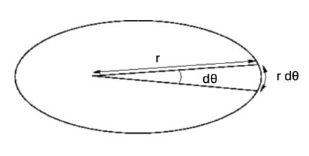
We can approximate the area traced out as the area of a triangle:
\[\begin{equation} dA = \frac{1}{2} r (r d\theta) \end{equation}\]Now we can take a time derivative of the expression above:
\[\begin{align} \frac{dA}{dt} &= \frac{\frac{1}{2} r (r d\theta)}{dt}\\[0.1cm] &= \frac{r^2}{2} \frac{d\theta}{dt}\\[0.1cm] &= \frac{r^2}{2} \dot{\theta}\\[0.1cm] &= \frac{r^2}{2} \frac{C}{r^2}\\[0.1cm] &= \frac{C}{2} \end{align}\]Thus, we have derived Kepler’s second law. The motion of the orbit traces out equal areas in equal times (since C is a constant).
Kepler’s First Law
Now that we know that C is the constant angular momentum of the system, we can take a closer look at the radial equation from above:
\[\begin{equation} r(\theta) = \frac{C^2}{GM \left [1 - ecos\theta \right ]} \end{equation}\]Just to simplify the expression, let \(p \equiv C^2/GM\). Then the equation becomes:
\[\begin{equation} r(\theta) = \frac{p}{1 - ecos\theta} \end{equation}\]But this is simply the equation for a conic section in polar form! The constant e defines the shape of the conic section. If \(e = 0\), the equation becomes:
\[\begin{equation} r(\theta) = \frac{p}{1} = p \end{equation}\]This means that the radius of the orbit is a constant value at every angle. In other words, the orbit is circular. If \(0 < e < 1\), then the shape of the orbit is an ellipse. The constant e represents the eccentricity of the orbit (i.e. how circular it is). If the eccentricity of the orbit is close to zero, the orbit is relatively circular. If the eccentricity of the orbit is close to one, the orbit traces out a very skinny ellipse. Thus, we see that the orbits are ellipses or circles (Kepler’s second law).
Remember, when \(e \ge 1\) the orbit traces out either a parabolic or hyperbolic arc. These are not bound orbits, so we will not focus on them here.
Kepler’s Third Law
We can use the information above to derive Kepler’s third law. First, we remember that the time derivative of the area traced out by an orbiting body is a constant:
\[\begin{equation} \frac{dA}{dt} = \frac{C}{2} \end{equation}\]We know that the period of the orbit is given by the total area traced out by the orbit (i.e. the area of an ellipse) divided by the time rate of change of the area:
\[\begin{equation} T = \frac{A}{\frac{dA}{dt}} \end{equation}\]The area of an ellipse is given by \(\pi a b\) where a and b are the major and minor radii of the ellipse. Then:
\[\begin{equation} T = \frac{2 \pi a b}{C} \end{equation}\]Then we can use the properties of an ellipse to simplify the expression:
\[\begin{equation} a = \frac{p}{1 - e^2} \end{equation}\] \[\begin{equation} b = \sqrt{1 - e^2} a \end{equation}\] \[\begin{equation} C = \sqrt{GMp} \end{equation}\]We will square the expression for the orbital period and plug in the equations above:
\[\begin{align} T^2 &= \frac{4 \pi^2 a^2 b^2}{C^2}\\[0.1cm] &= \frac{4 \pi^2 a^2 (1 - e^2) a^2}{GMp}\\[0.1cm] &= \frac{4 \pi^2 a^4 (1 - e^2)}{GM[a(1-e^2)]}\\[0.1cm] &= \frac{4 \pi^2 a^3}{GM}\\[0.1cm] \end{align}\] \[\begin{equation} T^2 = \frac{4 \pi^2 a^3}{GM} \end{equation}\]And this is Kepler’s Third Law. The period of the orbit squared is proportional to the major radius of the orbit cubed.
Conclusions
I think we have covered enough material to wrap up the topic of orbital motion for now. Hopefully the last three posts have given you a good background on the utility of reduced mass, the solution of the differential equation for an inverse squared law, and a derivation of Kepler’s laws. Of course this is just the beginning. Orbital motion is a rich area that I will return to in many later posts.
Until next week!