Reduced Mass and Binary Star Systems - Part 1
The Two-Body Problem
The concept of reduced mass is very useful in the field of classical mechanics; it is often used to simplify complicated problems that could not otherwise be solved. Suppose I am analyzing a two-body problem. Specifically, a point mass \(M_1\) has a position \(\vec{r}_1(t)\), and a point mass \(M_2\) has a position \(\vec{r}_2(t)\). The only force that will influence the path of the particles is the central force between them (e.g. gravitational force, Coulomb force, force of a harmonic oscillator, etc.). We can calculate the motion of each point mass using Newton’s second law:
\[\begin{equation} \vec{F}_{12} = M_1 \vec{a}_1 = M_1 \frac{d^2 \vec{r}_1}{dt^2} \end{equation}\] \[\begin{equation} \vec{F}_{21} = M_2 \vec{a}_2 = M_2 \frac{d^2 \vec{r}_2}{dt^2} \end{equation}\]In the expressions above, \(\vec{F}_{ij}\) is the force that particle j exerts on particle i. We will assume that the two objects are isolated, and thus, only feel the central force. Using Newton’s third law, we know that the forces must be equal and opposite: \(-\vec{F}_{12} = \vec{F}_{21}\). Let’s simplify the notation by calling the force \(\vec{F}\):
\[\begin{equation} -\vec{F} = M_1 \frac{d^2 \vec{r}_1}{dt^2} \end{equation}\] \[\begin{equation} \vec{F} = M_2 \frac{d^2 \vec{r}_2}{dt^2} \end{equation}\]Now, we have a pair of second-order, coupled, differential equations. Solving this system can be a bit tricky if we try to handle both of these expressions simultaneously. Luckily, there is an easy way to recast this problem and find a solution using reduced mass.
Reduced Mass
Let’s take a small detour. We can calculate the center of mass of this system:
\[\begin{equation} \vec{r}_{COM} = \frac{M_1 \vec{r}_1 + M_2 \vec{r}_2}{M_1 + M_2} \end{equation}\]And we can define the position vector connecting the two point masses \(M_1\) and \(M_2\):
\[\begin{equation} \vec{r} = \vec{r}_2 - \vec{r}_1 \end{equation}\]Now, we can rewrite \(\vec{r}_1\) and \(\vec{r}_2\) using the center of mass and \(\vec{r}\).
\[\begin{equation} \vec{r}_1 = \vec{r}_{COM} - \frac{M_2}{M_1 + M_2}\vec{r} \end{equation}\] \[\begin{equation} \vec{r}_2 = \vec{r}_{COM} + \frac{M_1}{M_1 + M_2}\vec{r} \end{equation}\]Let’s double check these expressions to make sure they are true. Checking \(\vec{r}_1\):
\[\begin{align} \vec{r}_1 &= \vec{r}_{COM} - \frac{M_2}{M_1 + M_2}\vec{r}\\[0.1cm] &= \frac{M_1 \vec{r}_1 + M_2 \vec{r}_2}{M_1 + M_2} - \frac{M_2}{M_1 + M_2}\vec{r}\\[0.1cm] &= \frac{M_1 \vec{r}_1 + M_2 \vec{r}_2}{M_1 + M_2} - \frac{M_2 \left ( \vec{r}_2 - \vec{r}_1 \right )}{M_1 + M_2}\\[0.1cm] &= \frac{M_1 \vec{r}_1 + M_2 \vec{r}_2 - M_2 \vec{r}_2 + M_2 \vec{r}_1}{M_1 + M_2}\\[0.1cm] &= \frac{M_1 \vec{r}_1 + M_2 \vec{r}_1}{M_1 + M_2}\\[0.1cm] &= \frac{M_1 + M_2}{M_1 + M_2} \vec{r}_1\\[0.1cm] &= \vec{r}_1 \end{align}\]And checking \(\vec{r}_2\):
\[\begin{align} \vec{r}_2 &= \vec{r}_{COM} + \frac{M_1}{M_1 + M_2}\vec{r}\\[0.1cm] &= \frac{M_1 \vec{r}_1 + M_2 \vec{r}_2}{M_1 + M_2} + \frac{M_1}{M_1 + M_2}\vec{r}\\[0.1cm] &= \frac{M_1 \vec{r}_1 + M_2 \vec{r}_2}{M_1 + M_2} + \frac{M_1 \left ( \vec{r}_2 - \vec{r}_1 \right )}{M_1 + M_2}\\[0.1cm] &= \frac{M_1 \vec{r}_1 + M_2 \vec{r}_2 + M_1 \vec{r}_2 - M_1 \vec{r}_1}{M_1 + M_2}\\[0.1cm] &= \frac{M_2 \vec{r}_2 + M_1 \vec{r}_2}{M_1 + M_2}\\[0.1cm] &= \frac{M_1 + M_2}{M_1 + M_2} \vec{r}_2\\[0.1cm] &= \vec{r}_2 \end{align}\]We can substitute these new expressions for \(\vec{r}_1\) and \(\vec{r}_2\) into Newton’s equations. The equation for \(\vec{r}_1\) becomes:
\[\begin{align} -\vec{F} &= M_1 \frac{d^2 \vec{r}_1}{dt^2}\\[0.1cm] &= M_1 \frac{d^2}{dt^2} \left [ \vec{r}_{COM} - \frac{M_2}{M_1 + M_2}\vec{r} \right ]\\[0.1cm] &= M_1 \left [ \frac{d^2 \vec{r}_{COM}}{dt^2} - \frac{M_2}{M_1 + M_2} \frac{d^2 \vec{r}}{dt^2} \right ]\\[0.1cm] \end{align}\]And the equation for \(\vec{r}_2\) becomes:
\[\begin{align} \vec{F} &= M_2 \frac{d^2 \vec{r}_2}{dt^2}\\[0.1cm] &= M_2 \frac{d^2}{dt^2} \left [ \vec{r}_{COM} + \frac{M_1}{M_1 + M_2}\vec{r} \right ]\\[0.1cm] &= M_2 \left [ \frac{d^2 \vec{r}_{COM}}{dt^2} + \frac{M_1}{M_1 + M_2} \frac{d^2 \vec{r}}{dt^2} \right ]\\[0.1cm] \end{align}\]Here we notice something crucial. This two-body system is isolated from all external forces and torques. The center of mass of the system does not accelerate. Thus, the second time derivative of the center of mass is zero. The expression for \(\vec{r}_1\) becomes:
\[\begin{align} -\vec{F} &= M_1 \left [ - \frac{M_2}{M_1 + M_2} \frac{d^2 \vec{r}}{dt^2} \right ]\\[0.1cm] \vec{F} &= \frac{M_1 M_2}{M_1 + M_2} \frac{d^2 \vec{r}}{dt^2}\\[0.1cm] \end{align}\]Similarly, the expression for \(\vec{r}_2\) becomes:
\[\begin{align} \vec{F} &= M_2 \left [ \frac{M_1}{M_1 + M_2} \frac{d^2 \vec{r}}{dt^2} \right ]\\[0.1cm] \vec{F} &= \frac{M_1 M_2}{M_1 + M_2} \frac{d^2 \vec{r}}{dt^2}\\[0.1cm] \end{align}\]We define \(\mu\) as the reduced mass of the system:
\[\begin{equation} \vec{F} = \mu \frac{d^2 \vec{r}}{dt^2} \end{equation}\] \[\begin{equation} \mu = \frac{M_1 M_2}{M_1 + M_2} \end{equation}\]Let’s look at the reduced mass more closely. Below, I have plotted the reduced mass as a function of \(M_1\). I have fixed \(M_2\) to be 1 kg.
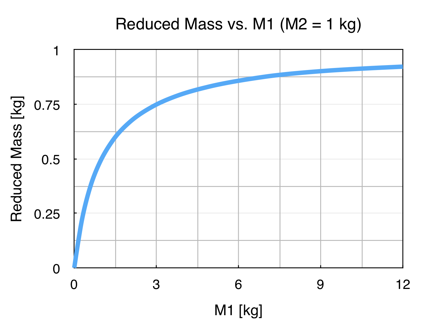
We see that when \(M_1\) is zero, the reduced mass is zero. As \(M_1\) becomes much larger than \(M_2\), the reduced mass approaches \(M_2\) (1 kg) but never quite reaches it. Thus, we see that the reduced mass is always less than either of the individual masses (which is why it is called reduced).
Binary Star Systems
The reduced mass is interesting, but how do we use it in an actual two-body problem? Let’s use the binary star system as an example. Most of the stars in our galaxy do not exist by themselves. Instead, they orbit around another star, and the pair travels through space. This setup is called a binary star system.
We will analyze the two stars as if they were two point masses traveling in space. Space is pretty empty, so we can assume that they are pretty well isolated from everything else around them. The only force that each star feels is the gravitational force from its partner:
\[\begin{equation} \vec{F} = - \frac{G M_1 M_2}{r^3} \vec{r} \end{equation}\]Let’s plug the gravitational force into the expression we derived above and see what we get:
\[\begin{align} \vec{F} &= \mu \frac{d^2 \vec{r}}{dt^2}\\[0.1cm] - \frac{G M_1 M_2}{r^3} \vec{r} &= \frac{M_1 M_2}{M_1 + M_2} \frac{d^2 \vec{r}}{dt^2}\\[0.1cm] - \frac{G}{r^3} \vec{r} &= \frac{1}{M_1 + M_2} \frac{d^2 \vec{r}}{dt^2}\\[0.1cm] - \frac{G\left ( M_1 + M_2 \right )}{r^3} \vec{r} &= \frac{d^2 \vec{r}}{dt^2}\\[0.1cm] \end{align}\]To simplify the expression, let the total mass of the two stars be \(M \equiv M_1 + M_2\):
\[\begin{equation} - \frac{GM}{r^3} \vec{r} = \frac{d^2 \vec{r}}{dt^2} \end{equation}\]Voila! What we see here is pretty great. We have taken a complicated pair of coupled differential equations and simplified it down to a single differential equation. Not only that, the final differential equation that we get is exactly the same as the one for a tiny satellite orbiting around a stationary massive planet. This is a problem we know how to solve!
Next week we will solve this equation and use it to determine some of the properties of the binary star system. See you then!